 |
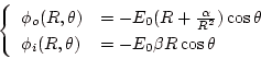
(1.24) |
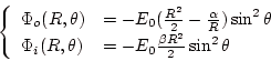 |
(1.25) |
gnuplot> set contour base
gnuplot> unset surface
gnuplot> set isosample 100
gnuplot> unset key
gnuplot> set view 0,0
gnuplot> set size square
gnuplot> set xrange [-2:2]
gnuplot> set yrange [-2:2]
gnuplot> set cntrparam levels incremental 0.05,0.1,3
gnuplot> mf(x,y)=x*x+y*y>1? sqrt(x*x*(1/2.0+2/5.0/(x*x+y*y)**1.5)): sqrt(x*x*3/10.0)
gnuplot> splot mf(x,y)
gnuplot> set output "sphere.eps"
gnuplot> set term postscript enhanced color eps
gnuplot> replot
gnuplot> set output "sphere_c.eps"
gnuplot> mf(x,y)=x*x+y*y>1? sqrt(x*x*(1/2.0+2/5.0/(x*x+y*y)**1.5)): sqrt(x*x*9/10.0)
gnuplot> replot
球内部では電場は一様なのでやはり(?)線密度も一様でないと
違和感があるということで等高線の密度を![]() の
等高線が等間隔になるようにプロットしている。
また、図1.12では誘電体の内外で電気力線が連続に
なるように
の
等高線が等間隔になるようにプロットしている。
また、図1.12では誘電体の内外で電気力線が連続に
なるように![]() ではなく
ではなく![]() の
等高線をプロット(あまり意味ないけど)。
の
等高線をプロット(あまり意味ないけど)。
![\includegraphics[width=7cm]{sphere.eps}](img131.png)
![\includegraphics[width=7cm]{sphere_c.eps}](img132.png)